Before the Main Contents
This post is Mike Lyou’s study notes of several courses, which cover thermodynamics, kinetics and some other knowledge. I do not own the copyright of some contents, if the article unintentionally infringes your copyright, it will be deleted shortly after being informed. All rights reserved.
This note is not complete, but will not be updated anymore, and may be deleted soon, because relavent course has ended. If you would like this post not being deleted, please let me know. Let me know if you notice any errors or typos, thanks so much.
Thermodynamics
1 Macroscopic Thermodynamics
1.1 Three levels of thermodynamics
There are three levels of thermodynamics.
-
The macroscopic or phenomenological description.
- It treats the matter as structureless.
- Macroscopic (equilibrium) thermodynamics describes and only describes equilibrium states.
- The statistical description.
- The quantum description.
1.2 Systems, Barriers and Surrounding
- System
- Barriers
- Diathermal or adiabatic
- Permeable or impermeable
- Movable or fixed
- Surrounding
1.3 Thermodynamic Variables
1.3.1 State variables and Process Variables
- State variables(or state functions): depends only on condition(or state) of the system. Eg. $V$, $S$, $T$, $U$, $H$, $G$.
- Process variables: quantities than only have meaning for changing systems. They are variable depending on the choice of path. Eg. $W$, $Q$.
1.3.2 Extensive and Intensive State Variables
The state variables can be classified into finer classes.
-
Extensive state variables: depend on system size. Which means double the system will change the variable value. Eg. $V$, $S$, $n$, $U$, $H$, $G$.
-
Intensive state variables: not depend on system size. Eg. $T$, $P$, $\mu$(chemical potemtial).
-
Normalized extensive variables *: extensive variables per mole or unit volume. These are in effect intensive. Eg. $v$, $s$.
$\rightarrow$ We’re more interested in intensive variables
$\rightarrow$ Many (Every?) extensive variable has a conjugate intensive variable. Common pairs are $(S,T)$, $(-P,V)$ and $(\mu,N)$. $\rightarrow$ See First Derivatives of Fundamental Equation for why they are conjugate.
2 Laws of Thermodynamic
2.1 Zeroth Law
If two systems are each in equilibrium with a third system, they are also in equilibrium with each other.
It describes the equilibrium.
2.2 First Law
Energy is conserved, it cannot be created or destroyed.
\[dU=\delta Q + \delta W + \delta W^\prime\]Where,
$dU$ means increase of internal energy,
$\delta Q$ means heat transferred into system,
$\delta W = -P dV$ is mechanical work,
$\delta W^\prime$ is sum of other works.
The first law is the law of energy.
2.3 Second Law
Entropy never decreases.
\[\mathrm{d} S \geqslant \frac{\delta Q}{T}\]where equal sign holds only for reversible process.
2.4 Third Law
The entropy of a thermodynamic system in internal equilibrium approaches a universal constant (usually taken as zero) as the absolute temperature goes to zero.
Which means entropy of any system at $T=0K$ is zero, no matter what values other system parameters are. It can be expressed as:
\[\left( \frac { \partial U } { \partial S } \right)_ { V, N_{1}, \ldots , N_{r} } = 0\]In the above equation, partial value is zero because $S \equiv 0$.
2.4.1 Calculation of entropy
According to the Third Law, the absolute value of entropy can be calculated.
For a reversible process
\[\mathrm{d} S = \frac{\delta Q}{T}\]and
\[\delta Q=C_{p} d T\]Therefore
\[S_T = S_0 + \int_{0}^T \frac{C_p}{T} dT = \int_0^T \frac{C_p}{T} dT\]or more practically
\[S_T = S_{298.15} + \int_{298.15}^{T} \frac{C_{p}}{T} d T\]3 Conditions of Equilibrium
3.1 Equilibrium States
Equilibrium states of simple macroscopic systems are characterized by system parameters including $\left( U, V, N_1, N_2, \cdots , N_r \right) $. If systems are more complex, parameters will be more.
The equilibrium states are states in which entropy is maximized for the given constraints.
3.2 The Fundamental Relation
The relation that gives the entropy as a function of the extensive parameters is known as the fundamental relation (in the entropic representation), which is
\[\boxed{S=S \left( U,V,N_1,N_2,\cdots N_r \right)}\]This relation is very useful.
-
If the fundamental relation of a system is known, all conceivable thermodynamic information about the system is ascertainable from it.
-
In other words, the information contained in the fundamental relation is thermodynamically all-inclusive.
3.3 Entropy of a Composite System
The entropy of a composite system has three important properties:
1. Additive over constituent subsystems
The entropy of a composite system is additive over the constituent subsystems, where the entropy of each subsystem is a function of the extensive parameters of that subsystem alone:
\[S=\sum_{\alpha} S^{(\alpha)} = \sum_{\alpha} S^{(\alpha)}\left(U^{(\alpha)}, V^{(\alpha)}, N_{1}^{(\alpha)}, \ldots, N_{r}^{(\alpha)}\right)\]The additive propertiey requires, that the entropy of a simple system is a homogeneous first-order function of the extensive parameters, or equavalent denoted as:
\[S\left(\lambda U, \lambda V, \lambda N_{1}, \dots, \lambda N_{r}\right)=\lambda S\left(U, V, N_{1}, \dots, N_{r}\right)\]2. Monotonically increase with respect to the energy
The monotonic property inplies that the partial derivative is positive. \(\left(\frac{\partial S}{\partial U}\right)_{V, N_{1}, \cdots, N_{r}}>0\)
We can know additionally, from this relation, that temperature is non-negative.
\[T \equiv \left(\frac{\partial U}{\partial S}\right)_{V, N_{1}, \cdots, N_{r}} = \left(\frac{\partial S}{\partial U}\right)_{V, N_{1}, \cdots, N_{r}} ^{-1}>0\]3. Continuous and differentiable The continuity, differentiability and monotonic properties together, imply that the entropy function can be inverted with respect to the energy. And the internal energy is single-valued, continuous and differentiable.
\[S=S\left(U, V, N_{1}, \cdots, N_{r}\right) \rightarrow U=U\left(S, V, N_{1}, \cdots ,N_{r}\right)\] \[\boxed{U=U\left(S, V, N_{1}, \cdots ,N_{r}\right)}\]Above is called the fundamental relation (in the energy representation).
Both of the two is the fundamental relation while in different forms, and each contains all thermodynamic information about the system.
\[S=S\left(U, V, N_{1}, \cdots, N_{r}\right) \leftrightarrow U=U\left(S, V, N_{1}, \cdots ,N_{r}\right)\]Because we are more interested in progress and changes in extensive parameters, we are more concerned with the energy representaton.
$\color{blue}{\text{(needs extention)}}$
3.4 First Derivatives of Fundamental Equation
Computing the first differential
\[d U=\left(\frac{\partial U}{\partial S}\right)_{V, N_{1}, \cdots, N_{r}} d S+\left(\frac{\partial U}{\partial V}\right)_{S, N_{1}, \cdots, N_{r}} d V+\sum_{j=1}^{r}\left(\frac{\partial U}{\partial N_{j}}\right)_{S, V_{N}, N_{r \neq j}} d N_{j}\]From the first differential we can obtain the first derivatives, which are defined as temperature $T$, pressure $P$, and chemical potential $\mu_j$.
\[\left(\frac{\partial U}{\partial S}\right)_{V, N_{1}, \cdots, N_{r}} \equiv T \\ \color{red}-\left(\frac{\partial U}{\partial V}\right)_{S, N_{1}, \cdots, N_{r}} \equiv P \\ \left(\frac{\partial U}{\partial N_j}\right)_{S, N_{1}, \cdots, N_{r\neq j}} \equiv \mu_j\]Notice that these partial derivatives are just the conjugate intensive functions of the corresponding extensive functions in the energetic representation.
Plugging them back, we have
\[d U=\color{blue}{T d S}-\color{green}{P d V}+\sum_{j=1}^{r}\mu_{j} d N_{j}\]Compare with the statement of the first law
\[dU=\color{blue}{\delta Q }+ \color{green}{\delta W_{mechanical}}+ \delta W_{chemical}\]$\color{blue}{\text{(result of the first law, or not?)}}$
3.5 Equation of State
Temperature, pressure and electrochemical potentials are partial derivatives of a function of $(\mathrm{S}, \mathrm{V}, \mathrm{N}{1}, \cdots \mathrm{N}{\mathrm{r}})$ and consequently are also functions of of $(\mathrm{S}, \mathrm{V}, \mathrm{N}{1}, \cdots \mathrm{N}{\mathrm{r}})$.
Thus, we have
\[\begin{aligned} &T=T\left(S, V, N_{1}, \dots, N_{r}\right)\\ &P=P\left(S, V, N_{1}, \dots, N_{r}\right)\\ &\mu_{j}=\mu_{j}\left(S, V, N_{1}, \dots, N_{r}\right) \end{aligned}\]These relations are called the equations of state. They express the intensive parameters in terms of extensive parameters.
Knowledge of a single equation of state does not constitute complete knowledge of the thermodynamic properties of the system, but knowledge of all the equations of state does.
Since the fundamental equation is homogeneous first order, it must be true that the equations of state are homogeneous zero order. We can represent this as
\[T\left(\lambda S, \lambda V, \lambda N_{1}, \ldots, \lambda N_{r}\right)=T\left(S, V, N_{1}, \ldots, N_{r}\right)\]The temperature of all systems is equal to the temperature of all subsystems (at equilibrium), this is the property an intensive function should have.
3.6 Conditions of Equilibrium
From the single fact that entropy is maximized for the given constraints, we can get several important implications.
3.6.1 Equilibrium of Temperature
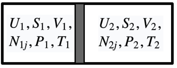
Now we have an isolated, composite system consisting of two simple systems. Two subsystems are separated by a wall that is rigid, impermeable, but allow the flow of heat.
Given the condition, we know that the volumes and mole numbers of each system are fixed. The only variables are energies of two subsystems, with the constrain of energy conservation
\[U^{(1)}+U^{(2)}=\text { constant } \quad \text{or} \quad dU^{(1)}+dU^{(2)}=0\]When the system has reached equilibrium, according to the definition of equilibrium, the entropy should reach its maximum. That is, a virtual transfer of energy from system 1 to system 2 will produce no change of entropy, i.e.
\[dS=0\]The entropy of the system is
\[S=S^{(1)}\left(U^{(1)}, V^{(1)} , N_{j}^{(1)}\right)+S^{(2)}\left(U^{(2)}, V^{(2)} , N_{j}^{(2)} \right)\]For better readability, here we use $N_j$ to represent $ N_{1},N_2,\cdots ,N_{r}$.
Since volumes and mole numbers are fixed, we can reresent the difference of entropy as
\[\begin{aligned} d S&=\left(\frac{\partial S^{(1)}}{\partial U^{(1)}}\right)_{V^{(1)},N_{j}^{(1)}} d U^{(1)}+\left(\frac{\partial S^{(2)}}{\partial U^{(2)}}\right)_{V^{(2)}, N_{j}^{(2)}} d U^{(2)}\\ &=\frac{1}{T^{(1)}} d U^{(1)}+\frac{1}{T^{(2)}} d U^{(2)}\\ &=\left(\frac{1}{T^{(1)}}-\frac{1}{T^{(2)}}\right) d U^{(1)} \end{aligned}\]Therefore
\[dS=0 \quad \Longrightarrow \quad T^{(1)}=T^{(2)}\]Q.E.D.
3.6.2 Equilibrium of Pressure
Similarly, if we have an isolated, composite system consisting of two simple systems. Two subsystems are separated by a wall that is impermeable, but moveable, and allow the flow of heat.
Upon this condition, the variables become energies and volumes of two subsystems. The only constants are mole numbers. And we can write
\[U^{(1)}+U^{(2)}=\text { constant } \quad \text{or} \quad dU^{(1)}+dU^{(2)}=0\] \[V^{(1)}+V^{(2)}=\text { constant } \quad \text{or} \quad dV^{(1)}+dV^{(2)}=0\]When the whole system has reached equilibrium, we have $dS=0$, and it can be expanded as
\[\begin{aligned} d S&=\left(\frac{\partial S^{(1)}}{\partial U^{(1)}}\right)_{V^{(1)},N_{j}^{(1)}} d U^{(1)} + \left(\frac{\partial S^{(1)}}{\partial V^{(1)}}\right)_{U^{(1)},N_{j}^{(1)}} d V^{(1)} \\ & +\left(\frac{\partial S^{(2)}}{\partial U^{(2)}}\right)_{V^{(2)}, N_{j}^{(2)}} d U^{(2)} + \left(\frac{\partial S^{(2)}}{\partial V^{(2)}}\right)_{U^{(2)}, N_{j}^{(2)}} d V^{(2)}\\ &=\frac{1}{T^{(1)}} d U^{(1)} + \frac{P^{(1)}}{T^{(1)}} d V^{(1)} + \frac{1}{T^{(2)}} d U^{(2)} + \frac{P^{(2)}}{T^{(2)}} d V^{(2)}\\ &=\left(\frac{1}{T^{(1)}}-\frac{1}{T^{(2)}}\right) d U^{(1)} + \left(\frac{P^{(1)}}{T^{(1)}}-\frac{P^{(2)}}{T^{(2)}}\right) d V^{(1)} \end{aligned}\]Now we know $dS=0$, then it must be true that
\[\left(\frac{1}{T^{(1)}}-\frac{1}{T^{(2)}}\right) = 0, \quad \left(\frac{P^{(1)}}{T^{(1)}}-\frac{P^{(2)}}{T^{(2)}}\right) = 0\]Therefore
\[dS=0 \quad \Longrightarrow \quad T^{(1)}=T^{(2)} \quad \Longrightarrow \quad P^{(1)}=P^{(2)}\]Q.E.D.
Ps1. Here we can prove wrong a possible mistake, which I have made before, that $dV^{(1)}+dV^{(2)}$ alone cannot derive the conclusion $P^{(1)}=P^{(2)}$.
Ps2. We can prove $(\partial S / \partial V)_ {U,N_j} \equiv P/T$ using jacobian.
3.6.3 Equilibrium of Chemical Potential
I dont wanna prove it since its similar to previous two.
3.7 Entropy Maximum Principle and Energy Minimum Principle
…
3.8 The Euler Equation
Ps. The pronunciation of Euler should be /ˈɔɪlər/. See wikipedia for more.
…
3.9 The Gibbs-Duhem Relation
…
4 Legendre Transformations, Thermodynamic Potentials and the Extremum Principle
Experimentally, we do not have an “entropymeter” to measure entropy, but instead we have the very useful and simple “thermometer” to measure temperature.
Also, experimentally it is often easier to do experiments at constant pressure rather than constant volume.
In other words, we would like the intensive, rather than the extensive, parameter(s) to be the independent variable(s).
4.1 Legendre Transform
For function $Y$ with a single independent variable $X$
\[\boxed{\begin{array}{c} Y=Y(X) \\ P={d Y}/{d X} \\ \psi=-P X+Y \\ \psi=\psi(P) \end{array}}\]And $\psi=\psi(P)$ is the Legendre transformed function of $Y=Y(X) $
\[Y=Y(X) \quad \rightarrow \quad \psi=\psi(P)\]Using the energy representation, the Legendre transformed functions are the thermodynamic potentials:
\[F=U-TS\] \[H=U+PV\] \[G=U-TS+PV\] \[\Xi = K = U - TS - \Sigma \mu N = -PV\]Where $\Xi$ is grand potential, equals Kramer potential $K$ (can be seen in HW10 and Lec18-page12).
4.2 The Extremum Principle
Here we will show, that the extremum principle for the thermodynamic potentials is one wherein the potential is minimized (for the given constraints).
Consider a composite system in diathermal contact with a heat reservoir (reversible heat source).
In the equilibrium state, the total internal energy of the composite system + the reservoir will reach its minimum:
\[\begin{aligned} &d\left(U+U^{r}\right)=0\\ &d^{2}\left(U+U^{r}\right)=d^{2} U>0 \end{aligned}\]Also, the total entropy will reach its maximum:
\[\begin{aligned} &d\left(S+S^{r}\right)=0\\ &d^{2}\left(S+S^{r}\right)=d^{2} S<0 \end{aligned}\]If the composite system is simple and comprises two subsystems 1 and 2, then we have
\[\begin{aligned} d\left(U+U^{r}\right) &=T^{(1)} d S^{(1)}+T^{(2)} d S^{(2)}+T^{r} d S^{r} \\ &=T^{(1)} d S^{(1)}+T^{(2)} d S^{(2)}-T^{r} d\left(S^{(1)}+S^{(2)}\right)=0\\ \therefore T^{(1)}=T^{(2)}&=T^{r} \end{aligned}\]Therefore, we can write
\[d\left(U+U^{r}\right)=d U+T^{r} d S^{r}=d U-T^{r} d S=0\] \[d \left(U-T^{r} S\right)=0 \tag{1}\]In addition, we can get this methematically:
\[d^2 \left(U-T^{r} S\right) = d^2U>0 \tag{2}\]Combining $(1)(2)$ we see, the minimum of inner energy or maximum of entropy also indicate the minimum of Helmholtz potential at equilibrium
\[F= U - T^r S\]Since the temperature of each subsystem is qual to temperature of reservoir, we can write it as
\[dF= d\left(U - T S\right)=0 \quad \text{(at equilibrium)}\]Known as Helmholtz Potential Minimum Principle.
Similarly, we can derive other principles:
Enthalpy minimum principle
...Gibbs free energy minimum principle
...4.3 Thermodynamics Potentials, Process and Work
Take Helmholtz free energy as our example again. We showed that $dF=0$ at equilibrium.
However, for any process that takes a system from an initial state to a final state, we can write for a small change in the state of the system
\[d F=d U-T d S-S d T\]Using the combination of first and second law
\[d U=T d S+\delta W_{\text{mechanical}}+\delta W_{\text{other}}\]We can write
\[d F=-S d T+\delta W_{\text{mechanical}}+\delta W_{\text{other}}\]Therefore we can arrive at the conclusion:
For isothermal processes, the Helmholtz free energy reports the total (reversible) work done on the system.
Similar for enthalpy $H$ and Gibbs free energy $G$ (E4201-hw8-2).
5 Second Derivatives of Fundamental Equation, Maxwell Relations, Stability
5.1 Useful Second Derivatives
These four five useful second derivatives should be remembered. They can sometimes serve as known values.
- Coefficient of thermal expansion
- Isothermal compressibility
- Adiabatic compressibility
- Molar heat capacity at constant pressure
- Molar heat capacity at constant volume
Ps. We can notice that they are partial derivatives of $V$ and $S$ with respect to $T$ and $V$ multiplied by other functions.
Attention: Not confuse $c_V$ with $C_V$ (which we nearly won’t see).
$c_V$ is molar heat capacity: $\Delta Q = n c_V \Delta T$ (where $n$ is mole number);
$C_V$ is specific heat: $\Delta Q = m c_V \Delta T$ (where $m$ is mass)
They are related by Avogadro number $N_{avo}$
\[c_V = C_V / N_{avo}\]
Additional relations (should be able to derive them):
\[c_{P}=c_{V}+\frac{T V \alpha^{2}}{N \kappa_{T}}\] \[\kappa_{T}=\kappa_{S}+\frac{T V \alpha^{2}}{N c_{P}}\]5.1.1 Derivation of Cp - Cv
By definition, we have
\[c_P - c_V = \frac{T}{N} \cdot \left[\left(\frac{\partial S}{\partial T}\right)_ {P, N} -\left(\frac{\partial S}{\partial T}\right)_ {V, N} \right]\]Plugging in the total differential of $S=S(V,T)$
\[dS = \left(\frac{\partial S}{\partial T}\right)_ {V,N} dT + \left(\frac{\partial S}{\partial V}\right)_ {T,N} dV\]We have
\[\left(\frac{\partial S}{\partial T}\right)_ {P,N} = \left(\frac{\partial S}{\partial T}\right)_ {V,N} \cdot 1 + \left(\frac{\partial S}{\partial V}\right)_ {T,N} \left(\frac{\partial V}{\partial T}\right)_ {P,N}\] \[\left(\frac{\partial S}{\partial T}\right)_ {V,N} = \left(\frac{\partial S}{\partial T}\right)_ {V,N} \cdot 1 + 0\]And therefore
\[c_P - c_V = \frac{T}{N} \cdot \left[\left(\frac{\partial S}{\partial V}\right)_ {T,N} \left(\frac{\partial V}{\partial T}\right)_ {P,N} \right]\]Simplify two derivatives inside
\[\left(\frac{\partial S}{\partial V}\right)_ {T,N} = \color{red}{+}\left(\frac{\partial P}{\partial T}\right)_ {V,N} = - \frac{\left(\frac{\partial V}{\partial T}\right)_ {P,N}}{\left(\frac{\partial V}{\partial P}\right)_ {T,N}} = -\frac{\alpha V}{-\kappa_T V} = \frac{\alpha}{\kappa_T}\] \[\left(\frac{\partial V}{\partial T}\right)_ {P,N} = \alpha V\]Plugging in to have
\[c_P - c_V = \frac{T}{N} \cdot \frac{\alpha}{\kappa_T} \cdot \alpha V = \frac{\alpha^2 TV}{\kappa_T N}\]Q.E.D (What is Q.E.D?)
5.2 Maxwell Relations
How to derive them
Derivation of Maxwell relations is simple. As an example, we have
\[dU=T dS - PdV + \mu dN\]And
\[\frac{\partial^{2} U}{\partial S \partial V}=\frac{\partial^{2} U}{\partial V \partial S}\]Therefore, we have
\[-\left(\frac{\partial P}{\partial S}\right)_ {V, N_{1}, N_{2}, \ldots}=\left(\frac{\partial T}{\partial V}\right)_ {S, N_{1}, N_{2}, \ldots}\]How to remember:
- Each pair of conjugate functions, e.g. $(S,T)$, sits at diagonal position.
- If $P$ involved, add a negative sign.
Because the conjugate $(-P,V)$ has a negative sign.
- If not all denominators are intensive (or all molecule are extensive) (e.g.$\partial T/ \partial V$), each exception gives one negative sign.
- Each molecule is the constant of the derivative across the equal sign.
You can find your own way to remember this, which is easiest to remember for you is the best.
5.3 Jacobian
See the supplementary document on Jacobians to help understand, which is more mathematical. Here we just list the results, which is enough for solving problems.
\[\boxed{ \begin{aligned} \left(\frac{\partial X}{\partial Y}\right)_ {Z} &=1 /\left(\frac{\partial Y}{\partial X}\right)_ {Z} \\ \left(\frac{\partial X}{\partial Y}\right)_ {Z} &=\left(\frac{\partial X}{\partial W}\right)_ {Z} /\left(\frac{\partial Y}{\partial W}\right)_ {z} \\ \left(\frac{\partial X}{\partial Y}\right)_ {Z} &= \color{red}{-}\left(\frac{\partial Z}{\partial Y}\right)_ {X} /\left(\frac{\partial Z}{\partial X}\right)_ {Y} \end{aligned} }\]Jacobians is very useful when we have e.g. $G,S$ as constant, and we want to bring it to denominators, so that we can either expand them or get the useful second derivatives.
5.4 Reduce the Derivatives (EP4)
General rules:
- Try to put extensive variables at molecule, and intensive variables at denominator. For example:
- Try to put expandable functions $(U,F,H,G)$ at molecule and expand them.
- Make use of the jacobians and Maxwell relationships when you need it.
- Be sure to remember all
fourfive second derivatives clearly.
- Plug in all results back and simplify it.
Ps. Not to confuse with this two:
\[\left(\frac{\partial \color{red}{T}}{\partial X}\right)_ {\color{red}{T}, N} \equiv 0, \quad \left(\frac{\partial \color{red}{T}}{\partial \color{red}{T}}\right)_ {X, N} \equiv 1\]
5.5 Stability
…
6 Unary Heterogeneous Systems
Unary: single component
Heterogeneous: more than one phase.
6.1 Phase
A phase is a physically distinct region of a system.
Different crystal structure means different phase, including allotropes (single component) and polymorphs (multicomponents).
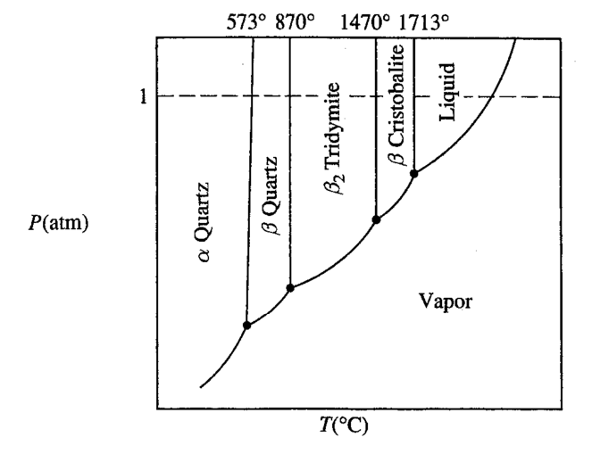
6.2 Phase Diagrams
Phase diagrams can tell us which phase id stable for a system under certain condition. Sometimes write for short as $\mathrm{PD}$ or $\mathrm{\Phi D}$.
2nd order phase cannot co-exist, but 1st order phase can.
6.3 Gibbs Phase Rule
Generally, the freedom of a system $F$, equals the numbers of variables minus numbers of independent relations. We can write it informally as
\[F = N_{\text{variables}} - N_{\text{relations}} \tag{1 }\]Consider a system composed of $C$ components and has $P$ phases.
In order to describe the composition of particular phase $\phi$, we need $(C-1)$ variables
\[\begin{equation*} x_i^\phi \quad (i=1,2,\cdots,C-1;\phi=\alpha,\beta,\delta,\cdots) \end{equation*}\]Here we don’t need the $C$-th variables, since it’s independent and can be determined via $\sum x_i^\phi = 1$.
Then for all $P$ phases we have $P(C-1)$ variables.
In addition, we treat temperature and pressure as variable for common thermodynamics systems, therefore there are two more variables. And in sum, we have
\[N_{\text{variables}} = P (C-1) + 2 \tag{2}\]As for the numbers of relations, we know that chemical potential of every component in each phase is equal in equilibrium, i.e.
\[\begin{equation*} \mu_i^\alpha = \mu_i^\beta = \mu_i^\delta = \cdots \quad (i=1,2,\cdots,C) \end{equation*}\]In sum
\(N_{\text{relations}} = C (P-1) \tag{3}\) Plugging $(2)(3)$ back to $(1)$, we have
\[\begin{aligned} F &= P (C-1) + 2 - C (P-1)\\ &= C-P+2 \end{aligned}\]The Gibbs Phase Rule
\[\boxed{F=C-P+2}\]If we are investigating condensed systems, the pressure can be considered fixed, therefore we have another representation
\[F=C-P+1\]$\rightarrow$ → Application of chemical reaction
6.4 The Clausius-Clapeyron Equation
A equilibrium line, where $\alpha$ and $\beta$ phases are in equilibrium, the $G, \mu, P,T$ must be equal, and therefore their viaration too $dG,d \mu, dP,dT$.
Then we have
\[\because d \mu^{\alpha}=d \mu^{\beta}\] \[\therefore -S^{\alpha} d T+V^{\alpha} d P=-S^{\beta} d T+V^{\beta} d P\] \[\therefore \frac{d P}{d T}=\frac{\Delta S^{\alpha \rightarrow \beta}}{\Delta V^{\alpha \rightarrow \beta}}\]Because
\[\Delta S^{\alpha \rightarrow \beta}=\frac{\Delta H^{\alpha \rightarrow \beta}}{T}\]If one of $\alpha$ and $\beta$ phases is gas phase, the volume of gas is much larger then condensed phase, using the ideal gas model
\[\Delta V^{\alpha \rightarrow {g}}=V^{g}-V^{\alpha} \approx V^{g}=\frac{R T}{P}\]Plugging in
\[\frac{d P}{d T}=\frac{\Delta H^{\alpha \rightarrow \beta}}{RT^2/P}\]Simplify it, we finally arrive at a very usefulrelation
\[\frac{d \ln P}{d T}=\frac{\Delta H^{\alpha \rightarrow \beta}}{RT^2}\]8 Binary Phase Diagrams
9 Multicomponent Homogeneous Nonreacting Systems: Solution
9.1 Partial Molar Properties (PMP)
Consider a multcomponent homogeneous system, with $c$ different components, each has mole number of $n_k ~ (k=1,2,…,c)$.
Attention:$~ ~ ~$ $n_k$ is mole number, not confuse with $N_k$ which is partical number. \(N_k= n_k \cdot N_{avo}(\text{Avogadro number}).\)
For an extensive thermodynamic property $\left(\mathrm{B}^{\prime}=\mathrm{U}^{\prime}, \mathrm{S}^{\prime}, \mathrm{V}^{\prime}, \mathrm{H}^{\prime}, \mathrm{G}^{\prime}, . .\right)$,
\[d B^{\prime}=\left(\frac{\partial B^{\prime}}{\partial T}\right)_ {P, n_{k}} d T+\left(\frac{\partial B^{\prime}}{\partial P}\right)_ {T, n_{k}} d P+\sum_{k=1}^{c} \color{red}{ \left(\frac{\partial B^{\prime}}{\partial n_{k}}\right)_ {T, P, n_{j} \neq n_{k}} } d n_{k}\]The partial molar property $B$ for component $k$ is then
\[\overline{B_{k}} \equiv\left(\frac{\partial B^{\prime}}{\partial n_{k}}\right)_ {T, P, n_{j} \neq n_{k}} \quad(k=1,2, \ldots,c)\]At constant temperature and pressure, we have
\[d B_{T, P}^{\prime}=\sum_{n_{k}=1}^{c} \overline{B_{k}} d n_{k}\]From full differential of $dB^\prime$ we know
\[d B^{\prime}=\sum_{k=1}^{c}\left[\overline{B_{k}} d n_{k}+n_{k} d \overline{B_{k}}\right]\]Combining above two equations, we get the Gibbs-Duhem Equation(Relation):
\[\boxed{\sum_{n_{k}=1}^{c} n_{k} d\overline{B_{k}} =0}\]9.2 Solution (Im’s Class)
Consider a solution made of two components:
\[\boxed{n_A \text{pure}A} + \boxed{n_B \text{ pure}B} \rightarrow \boxed{(n_A+n_B) ~(A+B\text{ solution})}\]The Gibbs free energy before and after mixing are:
\[G_{~seperate\\(or~before)}=n_A G_A^o+n_B G_B^o\] \[G_{~solution\\(or~after)}=n_A \overline{G_A}+n_B \overline{G_B}\]In which $G^o$ is Gibbs free energy of pure matter $\color{red}{(needs~ varify)}$, $\overline{G_A}$ is partial molar Gibbs free energy. They are both chemical potential, but little different.
\[G^o=\mu_A^o\] \[\overline{G_A}=\frac{\partial G_{solution}}{\partial n_A}=\mu_A\]Attention: Only in unary system $\mu \equiv g \equiv G$ (here $g=G/N$) . In multicomponent system $\mu_i = \partial G / \partial n_i $ for component $i$.
We can write the Gibbs-Duhem Equation
\[n_A d\overline{G_A}+n_B d\overline{G_B}=0\]For 1 mole solution, substituting in
\[x_A=\frac{n_A}{n_A+n_B} \quad x_B=\frac{n_B}{n_A+n_B}\]We have:
\[\boxed{ x_A d\overline{G_A}+x_B d\overline{G_B}=0 }\]And
\[\boxed{ G_{~seperate(or~before)}=x_A G_A^o+x_B G_B^o}\] \[\boxed{ G_{~solution(or~after)}=x_A \overline{G_A}+x_B \overline{G_B}}\]Now consider the Gibbs free energy change $\Delta G_{mix}$ before and after mixing, which should be:
\[\Delta G_{mix} = G_{solution} - G_{seperate}\]And then we can derive the following relations:
\[\Delta G_{mix} = \Delta H_{mix} - T \Delta S_{mix}\]or
\[\Delta G_{mix} = x_A \Delta \overline G_{mix, A}+x_B \Delta \overline G_{mix, B} = x_A (\overline{G_A}-G_A^o) + x_B (\overline{G_B}-G_B^o)\]Likewise
\[G_{sol} = H_{sol} - T \cdot S_{sol}\] \[G_{sol} = x_A \overline G_A + x_B \overline G_B \tag{* }\] \[G_{sol} = \Delta G_{mix} + G_ {seperate}\]Now we can construct the curve of $G_ {sol}$ for the first step.
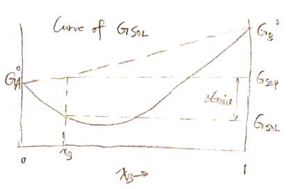
From $( * )$ we can derive
\[\frac{dG_{sol}}{dx_B} = - \overline G_A + \overline G_B\]And the tangent line at point $\left( x_B^\prime, G_{sol}\right)$ is then $G^\prime = G_{sol} + (x_B-x_B^\prime) \frac{dG_{sol}}{dx_B} $. Therefore we have the partial molar Gibbs free energy of $A$ and $B$:
\[\overline G_B = G_{sol} + (1-x_B)\frac{dG_{sol}}{dx_B}\] \[\overline G_A = G_{sol} + ~ ~ ~ ~ ~ x_B \cdot \color{red}{-}\frac{dG_{sol}}{dx_B}\]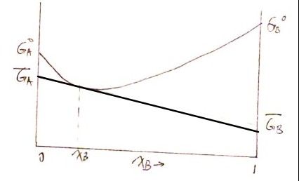
Plugging in activity $a$
\[\overline G_A = G_A^o +RT \ln a_A = \mu_A\]where
\[a_A = \gamma _A \cdot x_A = \frac{f_A}{f_A^o} \approx \frac{P_A}{P_A^o}\]In which, $\gamma_A$ is activity coefficient, $x_A$ is mole fraction of $A$.
This part seems to have collision with Prof. Barmak’s lecture, see Lec 9 Page 9.
Then we can expand $( * )$ to
\[\begin{aligned}G_{sol} ~&= x_A \overline G_A + x_B \overline G_B \\ &=x_A G_A^o +x_A RT \ln a_A + x_B G_B^o +x_B RT \ln a_B\\ &=\color{red}{\left(x_A G_A^o +x_B G_B^o \right) }+ \color{green}{RT \left(x_A \ln a_A + x_B \ln a_B \right)}\\ &=\color{red}{G_{sep}}\text{(known)}+ \color{green}{\Delta G_{mix}}\text{(conclusion)} \end{aligned}\]Then
\[\Delta \overline G_{mix, A} \equiv \frac{\partial \Delta G_{mix}}{\partial x_A} = RT \ln a_A = \overline G_A -G_A^o\\ \Delta \overline G_{mix, B} \equiv \frac{\partial \Delta G_{mix}}{\partial x_B} = RT \ln a_B = \overline G_B -G_B^o\]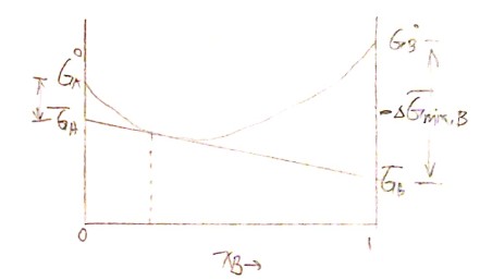
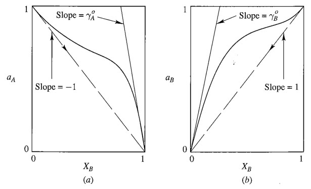
9.3 Binary Dilute solution
The solvent obeys Raoult’s Law
\[\lim_{X_A \rightarrow 1} a_A = X_A\]The solute obeys Henry’s Law
\[\lim_{X_B \rightarrow 0} a_B = \gamma^o X_B \\(\gamma^o:\text{Henry's Law constant})\]Here is an illustration from Prof. Barmak’s Lecture.
9.4 Ideal Solution
Assumption of ideal solution:
\[\boxed{ a_A = x_A, a_B = x_B} \quad (\text{i.e. } \gamma_A =\gamma_B =1)\]This assumption is derivated from ideal gas mixture, see Barmak’s Lec 9 Page 10.
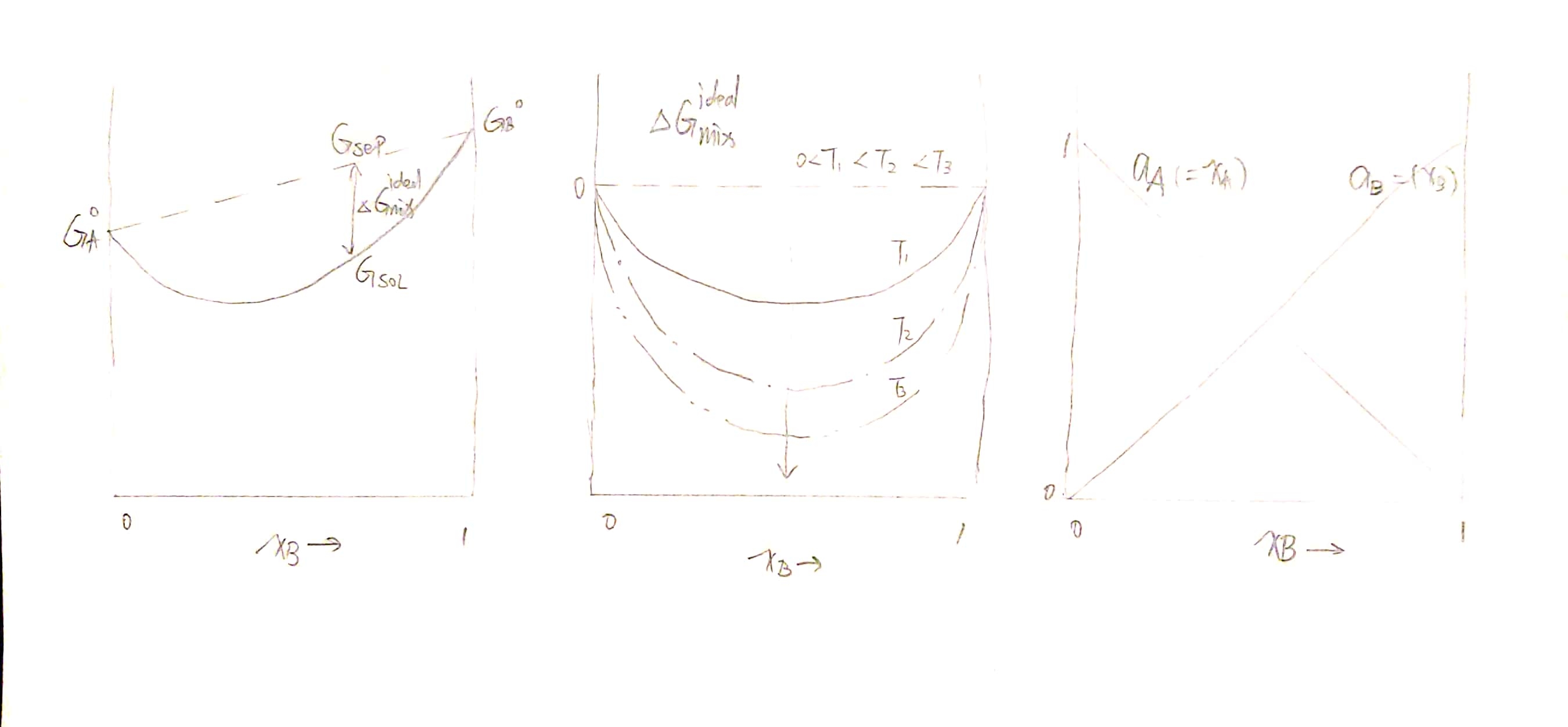
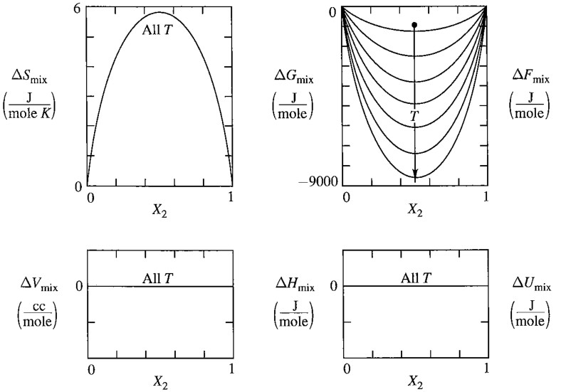
Upon this very simple assumption, we can derive
\[\Delta G_{mix}^{ideal} = RT \left[ x_A \ln x_A + x_B \ln x_B \right] \propto T\\ \Delta V_{mix}^{ideal} =\left(\frac{\partial \Delta G_{mix}^{ideal}}{\partial P}\right)_{T, x_B}=0\\ \Delta U_{mix}^{ideal} =\Delta H_{mix}^{ideal} = \left[\frac{\partial (\Delta G_{mix}^{ideal}/T)}{\partial (1/T)}\right]_{P, x_B} =0\]Noticing that $\Delta H_ {mix}^{ideal}=0$, we can conclude that $\Delta G_{mix}^{ideal} = -T \Delta S_ {mix}^{ideal}$, i.e.
\[\Delta S_{mix}^{ideal} = -R \left[ x_A \ln x_A + x_B \ln x_B \right]\]Here are two fine graphs:
9.5 Regular Solution
The difference of regular solution to ideal solution is, the enthalpy of regular solution is nonzero. $\color{red}{\text{needs varification}}$
Here we directly give the results:
\[\begin{aligned} \Delta G_{mix}^{reg} &= \Omega x_A x_B + RT \left[ x_A \ln x_A + x_B \ln x_B \right] \\ \Delta S_{mix}^{reg} &= \color{white}{zzzzzzzzzz}RT \left[ x_A \ln x_A + x_B \ln x_B \right] =\Delta S_{mix}^{ideal}\\ \Delta H_{mix}^{reg} &= \Omega x_A x_B \color{white}{zzzzzzzzzzzzzzzzzzzzzzzzzzzzz} \left(\Delta H_{mix}^{ideal} = 0 \right) \end{aligned}\]Regular solution will simplify to ideal solution when $\Omega = 0$
Attention: Nomenclature
In Im’s class, $\Omega$ is regular solution parameter, $\Omega = N_a \cdot z \left[ \epsilon_{AB} - \frac{1}{2} (\epsilon_{AA}+\epsilon_{BB})\right]$, $\omega$ is configurational entropy, $\omega = \frac{(N_A+N_A)!}{N_A! N_B!}$ .
While in Barmak’s class, the regular solution parameter is $a_0$, and configurational entropy is $\Omega$. Pay attention to this.
Using the “excess terms”, which means the difference with ideal solution
\[\Delta G_{mix}^{xs} = \Delta G_{mix} - \Delta G_{mix}^{ideal} \\ \Delta H_{mix}^{xs} = \Delta H_{mix} - \Delta H_{mix}^{ideal} \\ \Delta S_{mix}^{xs} = \Delta S_{mix} - \Delta S_{mix}^{ideal}\]For regular solution, we can prove that
\[\Delta G_{mix}^{xs,~reg} = \Omega ~ x_A x_B \\ \Delta H_{mix}^{xs,~reg} = \Omega ~ x_A x_B \\ \Delta S_{mix}^{xs,~reg} = 0 \color{white}{zzzzzz}\]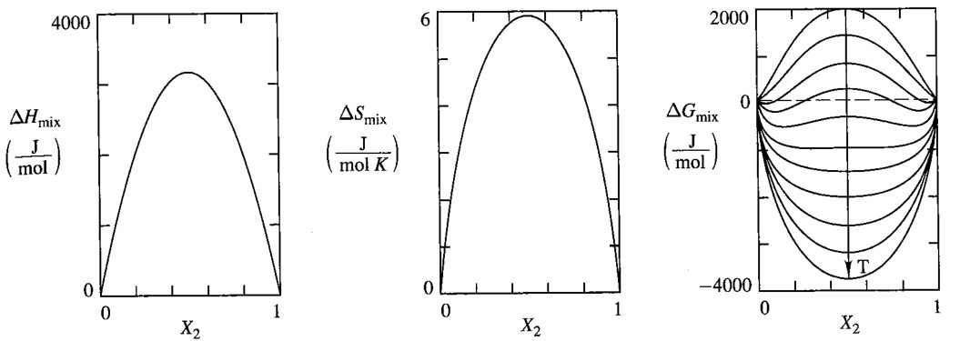
9.5.1 Regular Solution Parameter
Consider 1 mole solid solution made of atoms A and B, with mole fraction of $x_A$ and $x_B$. And we want to investigate the enthalpy change during the mixing process $\Delta H_{mix}$
\[\Delta H_{mix} = H_{\text{solution}} - H_{\text{initial}}\]Because solid solution is a condensed system, the enthalpy is approximately equal to energy, which can be expressed in terms of bound energies:
\[\Delta H_{mix} \approx E_{\text{solution}} - E_{\text{initial}} \tag{1}\]For intial state,
\[E_{\text{initial}} = x_A E_A^o + x_B E_B^o\]where $E_A^o$ is energy of 1 mole pure A, and $E_B^o$ is energy of 1 mole pure B:
\[E_A^o = \frac{ N_{avo}Z}{2} \epsilon_{AA} \quad E_B^o = \frac{ N_{avo}Z}{2} \epsilon_{BB}\]in which, $N_{avo}$ is Avogadro’s number, $Z$ is coordination number(number of nearest neighbors), and we assume the coordination number is same for A, B and AB solution. $\epsilon_{AA}$ and $\epsilon_{BB}$ are bound energies of A-A bound and B-B bound.
Therefore the total energy before mixing is
\[E_{\text{initial}} = \left[ x_A \epsilon_{AA} +x_B \epsilon_{BB} \right] \frac{ N_{avo}Z}{2} \tag{2}\]For solid solution
\[E_{\text{solution}} = P_{AA}\epsilon_{AA} + P_{BB}\epsilon_{BB} + P_{AB}\epsilon_{AB}\]where $P_{AA}, P_{BB},P_{AB}$ are numbers of A-A, B-B and A-B bounds.
Because of an important assumption of regular solution, that atoms are mixed randomly, we have
\[P_{AA} = \frac{ N_{avo}Z}{2}\] \[P_{BB} = x_B x_B \frac{ N_{avo}Z}{2}\] \[P_{AB} = 2 \cdot x_A x_B \frac{ N_{avo}Z}{2}\]Then substitute to get total energy after mixing
\[E_{\text{solution}} = \left[ x_A^2 \epsilon_{AA} +x_B^2 \epsilon_{BB} + 2 x_A x_B \epsilon_{AB}\right] \frac{ N_{avo}Z}{2} \tag{ 3}\]Plugging $(2)(3)$ into $(1)$
\[\begin{aligned} \Delta H_{mix} &\approx \frac{ N_{avo}Z}{2} \left[ (x_A \epsilon_{AA} +x_B \epsilon_{BB} ) -(x_A^2 \epsilon_{AA} +x_B^2 \epsilon_{BB} + 2 x_A x_B \epsilon_{AB}) \right]\\ &= \frac{ N_{avo}Z}{2} x_A x_B\left[ 2 \epsilon_{AB} - \epsilon_{AA} - \epsilon_{BB}\right] \\ &= \Omega x_A x_B \end{aligned}\]where
\[\Omega = N_{avo}Z\left[ \epsilon_{AB} - \frac{1}{2}(\epsilon_{AA} - \epsilon_{BB})\right]\]9.6 Nonregular(Subregular or Real) Solution
For component $A$, we have
\[\Delta \overline G_{mix,~A}^{xs,~real} = \Delta \overline G_{mix,~A}^{real} - \Delta G_{mix,~A}^{ideal} = RT \ln \gamma_A\]Therefore for the whole solution, we have
\[\begin{aligned} \Delta G_{mix}^{xs,~real} &= \Delta G_{mix}^{~real} - \Delta G_{mix}^{ideal} = RT \left[ x_A \ln \gamma_A + x_B \ln \gamma_B\right] \\ \Delta G_{mix}^{xs}&= \Delta H_{mix}^{xs} - T \Delta S_{mix}^{xs} \end{aligned}\]Since we already know $\Delta H_{mix}^{ideal} = 0$, $\Delta V_{mix}^{ideal} = 0$, then we know
\[\Delta H_{mix}^{xs,~real} = \Delta H_{mix}\\ \Delta V_{mix}^{xs,~real} = \Delta V_{mix}\]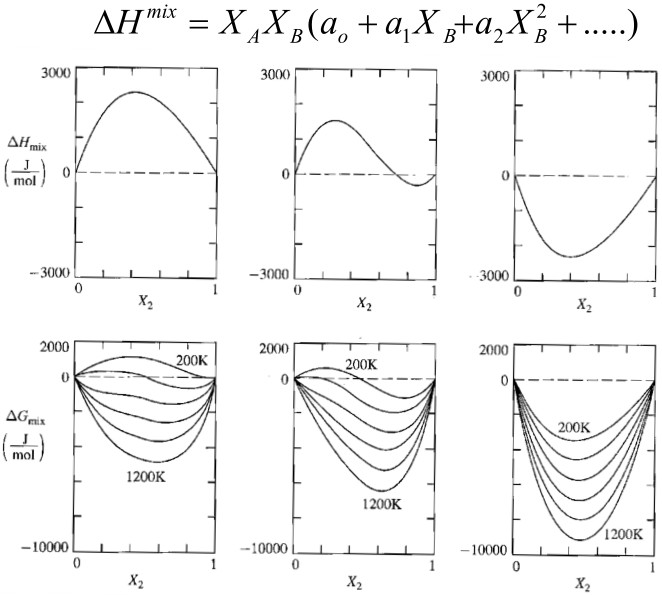
14 Electrochemistry
Pro. Barmak’s electrochemistry may be different from E4260. If there are any difference, use the version of Pro. Barmak’s.
14.1 Equilibrium in Weak Electrolytres
\[c_{k}=[k]=\frac{X_{k}}{V}\]where $c_k$ is molar concentration, $[k]$ is molarity (mole number of component $k$ per liter of solution), $X_k$ is mole fraction of component $k$, $V$ is molar volume of solution.
\[a_{k}=f_{k} c_{k}=f_{k}[k]\] \[f_k = \gamma_k V\]$a_k$ is avtivity of $k$, $\gamma_k$ is activity coefficient.
To fing the condition for equilibrium, we have to consider all reactions in the solution.
For water,
\[H_{2} O=H^{+}+O H^{-}\] \[A_{w}=\left(\mu_{H^{+}}+\mu_{O H^{-}}\right)-\mu_{H_{2}O} \quad\text{(affinity)}\] \[\Delta G_{w}^{o}=-R T \ln K_{w}\] \[K_{w}=\frac{a_{H^{+}} a_{O H^{-}}}{a_{H_{2} O}}\]By the way, $\mathrm{pH}$ is defined by
\[\mathrm{pH}=-\log a_{H^+} = -\log [H^+]\] \[\mathrm{pOH}=-\log a_{OH^-} = -\log [OH^-]\] \[\mathrm{pH} + \mathrm{pOH} = 14 \quad \text{(at room temperature)}\]For compound,
\[M_{u} X_{v}=u M^{z+}+v X^{z-}\] \[A_{C}=\left(u \mu_{+}+v \mu_{-}\right)-\mu_{U}\] \[\Delta G_{C}^{o}=-R T \ln K_{C}\] \[K_{C}=\frac{a_{+}^{u} a_{-}^{v}}{a_{U}}=\frac{f_{+}^{u} f_{-}^{v}}{f_{U}} \frac{\left[M^{z+}\right]^{u}\left[X^{z-}\right]^{u}}{\left[M_{u} X_{v}\right]}\] \[K_{C}=K_{f} \frac{\left[M^{z+}\right]^{u}\left[X^{z-}\right]^{u}}{\left[M_{u} X_{v}\right]}\]We usually define the reference state so that in dilute solution, $K_f=1$.
For weak electrolytes, introduce the degree of dissociation, $\alpha$ ($\alpha \ll 1$ for week electrolytes) and the total concentration of the electrolyte compound added to make the solution, $c_C$
\[\begin{aligned} &\left[M^{z+}\right]=u \alpha c_{c} ; \quad\left[X^{z-}\right]=v \alpha c_{c} ; \quad\left[M_{u} X_{v}\right]=(1-\alpha) c_{c}\\ &K_{C}=\frac{\left(u \alpha c_{C}\right)^{u}\left(v \alpha c_{C}\right)^{v}}{(1-\alpha) c_{C}}=u^{u} v^{v} \frac{\alpha^{(u+v)} c_{C}^{(u+v-1)}}{(1-\alpha)} \end{aligned}\]14.2 Equilibrium in Strong Electrolytres
In dilute solutions, strong electrolytes are fully dissociated, i.e. $\alpha=1$
14.3 Equilibrium in a Two-Phase System Involving an Electrolyte
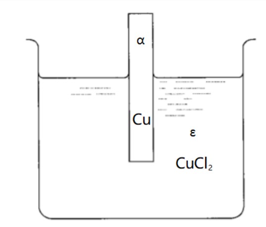
The reaction is: $C u^{\alpha}=\left(C u^{2+}\right)^{\varepsilon}+2\left(e^{-}\right)^{\alpha}$
Components in $\alpha$ phase: $C u, e^{-} $
Components in $\varepsilon$ phase: $\left(C u^{2+}\right)^{\varepsilon},\left(C l^{-}\right)^{\varepsilon}, C u C l_{2}, H^{+}, O H^{-}, H_{2} O$
Electrical potential of two phases: $\phi^\alpha, \phi^\varepsilon$
After a long derivation ↓
\[d S^{\prime \alpha}=\frac{1}{T^{\alpha}} d U^{\prime \alpha}+\frac{P^{\alpha}}{T^{\alpha}} d V^{\prime \alpha}-\frac{1}{T^{\alpha}}\left[\mu_{C u}^{\alpha} d n_{C u}^{\alpha}+\mu_{e}^{\alpha} d n_{e}^{\alpha}\right]\] \[d S^{\prime \varepsilon}=\frac{1}{T^{\varepsilon}} d U^{\prime \varepsilon}+\frac{P^{\varepsilon}}{T^{\varepsilon}} d V^{\prime \varepsilon}-\frac{1}{T^{\varepsilon}} \mu_{C u^{2+}}^{\varepsilon} d n_{C u^{2+}}^{\varepsilon}\] \[d S_{s y s}^{\prime}=d S^{\prime \alpha}+d S^{\prime \varepsilon}\]Isolation constraints:
\[d m_{C u}=0=d n_{C u}^{\alpha}+d n_{C u^{2+}}^{\varepsilon}\] \[d q_{t o t}=0=d q^{\alpha}+d q^{\varepsilon}=(-1) F d n_{e}^{\alpha}+(+2) F d n_{C u^{2+}}^{\varepsilon}\]Additional isolation constraints:
\[d V_{s y s}^{\prime}=0=d V^{\prime \alpha}+d V^{\prime \varepsilon}\] \[d U_{T o t}^{\prime}=0=d U^{\prime \alpha}+d U^{\prime \varepsilon}+\phi^{\alpha} d q^{\alpha}+\phi^{\varepsilon} d q^{\varepsilon}\] \[d U_{T o t}^{\prime}=0=d U^{\prime \alpha}+d U^{\prime \varepsilon}+\phi^{\alpha}\left(-F d n_{e}^{\alpha}\right)+\phi^{\varepsilon}\left(z^{+} F d n_{C u^{2+}}^{\varepsilon}\right)\]Use all expressions to arrive at:
\[d S_{\text {sys,isolated }}^{\prime}=\left(\frac{1}{T^{\alpha}}-\frac{1}{T^{\varepsilon}}\right) d U^{\prime \alpha}+\left(\frac{P^{\alpha}}{T^{\alpha}}-\frac{P^{\varepsilon}}{T^{\varepsilon}}\right) d V^{\prime \alpha} \quad\] \[-\frac{1}{T^{\alpha}}\left[\mu_{C u}^{\alpha}-2 \mu_{e}^{\alpha}-\mu_{C u^{2}+}^{\varepsilon}+2 F\left(\phi^{\alpha}-\phi^{\varepsilon}\right)\right] d n_{C u}^{\alpha}\] \[T^{\alpha}=T^{\varepsilon}, \quad P^{\alpha}=P^{\varepsilon}\]↓We eventually arrive at this:
\[\mu_{C u}^{\alpha}-2 \mu_{e}^{\alpha}-\mu_{C u^{2+}}^{\varepsilon}=-2 F\left(\phi^{\alpha}-\phi^{\varepsilon}\right)\]The application of this relation is obtaining $\phi^{\alpha}-\phi^{\varepsilon}$ by measuring $\mu_{C u}^{\alpha}-2 \mu_{e}^{\alpha}-\mu_{C u^{2+}}^{\varepsilon}$.
14.4 Equilibrium in an Electrochemical Cell
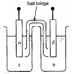
Take $\mathrm{Cu-Zn}$ battery as a concrete example.
The reactions are
\[\begin{aligned} &\left(C u^{2+}\right)^{\varepsilon}+2\left(e^{-}\right)^{\alpha}=C u^{\alpha}\\ &\left(Z n^{2+}\right)^{\eta}+2\left(e^{-}\right)^{\beta}=Z n^{\beta} \end{aligned}\]Conditions of equilibrium
\[\begin{aligned} &\mu_{C u}^{\alpha}-\left(2 \mu_{e}^{\alpha}+\mu_{C u^{2+}}^{\varepsilon}\right) =-2 F\left(\phi^{\alpha}-\phi^{\varepsilon}\right)\\ &\mu_{Zn}^{\beta}-\left(2 \mu_{e}^{\beta}+\mu_{Z n^{2+}}^{\eta}\right)=-2 F\left(\phi^{\beta}-\phi^{\eta}\right)\\ &\phi^{\varepsilon}=\phi^{\eta} \quad \text{(After connecting the salt bridge)}\\ &\mu_e^\beta = \mu_e^\alpha \quad \text{(After connecting the external cuicuit)} \end{aligned}\]Combining the up four relations, we find
\[\boxed{[\mu_{Z n}^{\beta}-\mu_{Zn^{2+}}^{\varepsilon}] - [\mu_{Cu}^{\alpha}-\mu_{Cu^{2+}}^{\varepsilon}] = -2 F\left(\phi^{\beta}-\phi^{\alpha}\right)}\]And overall cell reaction is
\[Z n^{\beta}+\left(C u^{2+}\right)^{\varepsilon}=C u^{\alpha}+\left(Z n^{2+}\right)^{\varepsilon}\]14.5 Conditions for Equilibrium in a General Galvanic Cell
Several conventions in this class:
- Write the affinities for the reduction reactions
-
The electromotive force (emf) for the cell is then the potential of the right electrode minus that for the left.
-
Rules of writing cell notations (copied from E4260 notes):
- Oxidation on the left, reduction on theright (in galvanic mode).
- A line as phaseboundary.
- Double line indicates a salt bridge: two interfaces.
- Metal electrodes at two ends.
14.6 Temperature Dependence of the Electromotive Force for a Cell
\[\begin{array}{l} \Delta S^{o}=-\left(\frac{\partial \Delta G^{o}}{\partial T}\right)_{P, n_{k}}=+z F\left(\frac{\partial E^{o}}{\partial T}\right)_{P, n_{k}} \\ \Delta H^{o}=\Delta G^{o}+T \Delta S^{o}=z F\left[E^{o}+T\left(\frac{\partial E^{o}}{\partial T}\right)_{P, n_{k}}\right] \end{array}\]
So?
14.7 The Standard Hydrogen Electrode (SHE)
(From E4260) Normal hydrogen electrode (NHE) $E^o=0$
For convience, we usually use standerd hydrogen electrode (SHE) instead of NHE.
14.8 Pourbaix Diagrams
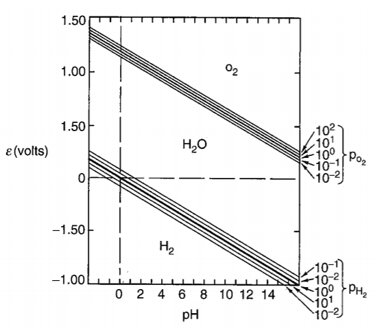
At upper region, oxygen is liberated from water; at bottom region, hydrogen is liberated from water.
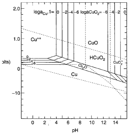
Above a line, oxygen is liberated from water; below b line, hydrogen is liberated from water.
Vertival line relates with reactions that no electrons involved.
Hrizontal line relateds with reactions that no H+ involved.
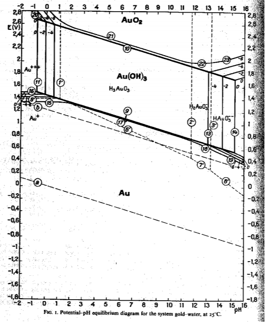
Water lines a and b fall within the neutral gold, Au, region. It is consistent with our common knowledge that gold is stable.
15 Point Defects in Metals
15.1 Defect Types
- 0-D, point defects
- 1-D, line defects (dislocations)
- 2-D, planar defects (surfaces, grain boundaries, interphase interfaces)
- 3-D, volume defects (voids)
15.2 Vacancies in Elemental Materials
Formation of vacancies requires expenditure of energy to break bonds, but results in increased entropy.
Vacancies are entropically stabilized and, as a result, there are always some vacancies present when a material is in equilibrium, i.e., vacancies are equilibrium defects.
15.3 Conditions for Equilibrium in a Crystal with Vacancies
After a long derivation
Consider a system composed of a homogeneous crystalline phase (α) and it vapor (g)
Variation of the entropy of this combined system is given by
\[\begin{aligned} d S_{s y s}=& \frac{1}{T^{\alpha}} d U^{\prime \alpha}+\frac{P}{T^\alpha} d V^{\prime \alpha}-\frac{1}{T^\alpha} \sum_{k=1}^{c} \mu_{k}^{\alpha} d n_{k}^{\alpha}-\frac{1}{T} \mu_{v}^{\alpha} d n_{v}^{\alpha} \\ & \frac{1}{T^{g}} d U^{\prime g}+\frac{P}{T^{g}} d V^{\prime g}-\frac{1}{T^{g}} \sum_{k=1}^{c} \mu_{k}^{g} d n_{k}^{g} \end{aligned}\]For the composite system isolated from its surroundings, we will have:
\[\begin{array}{l} d U_{s y s}^{\prime}=0=d U^{\prime \alpha}+d U^{\prime g} \\ d V_{s y s}^{\prime}=0=d V^{\prime \alpha}+d V^{\prime g} \\ d n_{k, s y s}=0=d n_{k}^{\alpha}+d n_{k}^{g} \end{array}\]Note that number of atomic sites and vacancies are not constrained in isolated system, since we can move an atom from the interior to its surface and vice versa.
Insert the isolation conditions into the entropy variation for the system to arrive at
\[d S_{\text {sys,isolated }}=\left(\frac{1}{T^{\alpha}}-\frac{1}{T^{g}}\right) d U^{\prime\alpha}+\left(\frac{P^{\alpha}}{T^\alpha}-\frac{P^g}{T^g}\right) d V^{\prime \alpha}-\sum_{k=1}^{c}\left(\frac{\mu_{k}^{\alpha}}{T^\alpha}-\frac{\mu_{k}^{g}}{T^{g}}\right) d n_{k}^{\alpha}-\frac{\mu_{v}^{\alpha}}{T^\alpha} d n_{v}^{\alpha}\]In this equation, $n_\nu$ is an independent variable because atomic sites may be created or annihilated with no other changes in the system.
At =m, entropy is maximized, and so in addition to the familiar conditions for equality of temperature, pressure and chemical potentials of the components of the solid phase, α, and the vapor phase, we will have
\[\boxed{\mu_\nu^\alpha = 0}\]Which means in a crystal at =m, the chemical potential of vacancies is zero.
15.4 Vacancy Concentration in Elemental Crystal at Equilibrium
To calculate this, we can consider the non-perfect crystal as a dilute solution, with atoms as solvent and vacancies as solute. Then the chemical potential of any component is partial molar Gibbs free energy, write as:
\[\mu_v^\alpha = \overline G_v^\alpha = \overline H_v^\alpha-T(\overline S_v^{xs,\alpha}+S_v^{ideal,\alpha})=0\] \[S_v^{ideal,\alpha} = -k \ln X_v^\alpha\]Therefore the concentration of vacancy is:
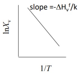
\[X_v^\alpha = \exp \left[\frac{\bar{S}_{v}^{x s, \alpha}}{k}\right] \exp \left[-\frac{\bar{H}_{v}^{\alpha}}{k T}\right]\]or
\[\boxed{X_v^\alpha = \exp \left[\frac{\Delta S_v^f}{k}\right] \exp \left[-\frac{\Delta H_v^f}{k T}\right]}\]Where $\Delta S_v^f$ is formation entropy of vacancies, and $\Delta H_v^f$ is formation enthalpy of vacancies.
15.5 Experimental Proof of Vacancies
Measure relative change in length, $∆L/L$ and relative change in lattice parameter, $∆a/a$, as a function of temperature
Thermal expansion contributes to both change in length and change in lattice parameter.
Creation of vacancies contributes to change in length, but not to the change in lattice parameter.
Mono-Vacancy concentration is proportional to
\[3\left(\frac{\Delta L}{L}-\frac{\Delta a}{a}\right)\]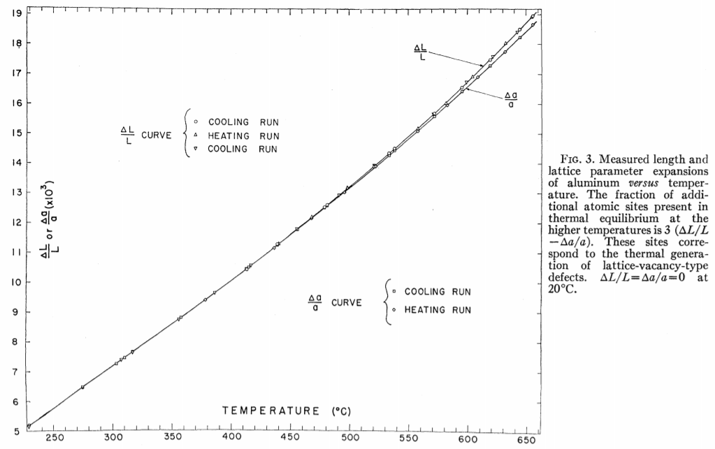
R. O. Simmons and R. W. Balluffi, Phys. Rev. 117, 52-60 (1960).
15.6 Self Interstitials and Frenkel Defects
Self Interstitials: follow the same line of reasoning, but here take atom from surface and insert into an interstitial site.
Note that formation energy of self-interstitial is 2- 4 times that for the vacancy. Therefore, the concentration of self-interstitials is many orders of magnitude smaller than for vacancies.
Like vacancies, self-interstitials are intrinsic point defects and their presence results in a volume change (reduction) relative to that for thermal expansion.
A Frenkel defect is a vacancy-interstitial pair
15.7 Solutes and Impurities
Element or elements dissolved in the host are solutes (when wanted) or impurities (when not wanted)
- Substitutional
- Interstitial
Are extrinsic defects.
Their =m concentration is determined by alloy thermodynamics.
The following content is from Beiley’s class.
Impurities can be further classified into two types: substitutional (usually for larger atoms) and imputities (usually for smaller stoms).
Hume-Rothery rules: Conditions usually satisfied for complete solid solubility
- Same crystal structure for pure A and pure B
- Difference in atomic radii $r_A$, $r_B$ small (max 10%)
- No difference in electronegativities
15.8 A Summary

16 Point Defects in Ionic Compounds
16.1 Defect Type
Defects in ionic compounds can be ionic or electronic:
-
Ionic defects: Occupy atomic positions in the crystal, which can be vacancies, interstitial ions, substitutional ions, impurities, or ions on the wrong sites (antisite defects)
-
Electronic defects: Deviations from a ground state electron orbital configuration give rise to such defects when valence electrons are excited into higher energy orbitals/levels and lead to formation of electron or holes.
Usually, point defects in metals are electrically neutral whereas in ionic compounds point defects are electrically charged.

→ The high mobility of the ionic defects in certain compounds makes them suitable candidates as solid electrolytes for batteries and fuel cells.
16.2 Kröger-Vink Notation
Because points defects in ionic compounds are usually charged, we need a set of notations to indicate this charge. Therefore we here introduce the Kröger-Vink Notation.
The Kröger-Vink notation allows us to identify:
- the defect type
- the site on which the defect is located
- the effective charge of the defect relative to the charge on the given site in a perfect crystal (or in a chosen reference crystal)
General form is:
\[M_S^C\]In which,
-
$M$ corresponds to structure element, can be atoms (e.g. Si, Ni), vacancies ($v$), interstitials ($i$), electrons ($e$) or electron holes ($h$).
-
$S$ indicates the lattice site that the species occupies, including interstitials.
-
$C$ corresponds to the electronic charge of the species relative to the site that it occupies. Prime($\prime$) denotes negative charge, dot ($\bullet$) denotes positive charge, star ($ \ast $)denotes neutrality, two dots indicate double positive charge.
Examples in $\mathrm{NaCl}: \mathrm{Na^+ Cl^-}$
| Kröger-Vink Notation | Meaning |
|---|---|
| $\mathrm{Na}\mathrm{Na}^\ast$ ,$\mathrm{Cl}\mathrm{Cl}^\ast$ | Atroms in NaCl perfect crystal |
| $v_\mathrm{Na}^\prime$ , $v_\mathrm{Cl}^\bullet$ | Vacancies (A vacancy on the sodium site has a charge of -1 relative to the sodium site in the perfect crystal) |
| $\mathrm{Na}_i^\bullet$ ,$\mathrm{Cl}_i^\prime$ | Interstitials |
| $\mathrm{Ca}\mathrm{Na}^\bullet$,$\mathrm{K}\mathrm{Na}^\ast$ | Aliovalent and isovalent (what?) |
Examples in $\mathrm{Y_2O_3}: \mathrm{Y^{3+} O^{2-}}$
| Kröger-Vink Notation | Meaning |
|---|---|
| $\mathrm{Y}\mathrm{Y}^\ast,\mathrm{O}\mathrm{O}^\ast$ | Atroms in perfect $\mathrm{Y_2O_3}$ crystal |
| $v_\mathrm{Y}^{\prime\prime\prime},v_\mathrm{O}^{\bullet\bullet}$ | Vacancies |
| $\mathrm{Y}_i^{\bullet\bullet\bullet},\mathrm{O}_i^{\prime\prime}$ | Interstitials |
| $\mathrm{Mg}_\mathrm{Y}^\prime$ | Aliovalent |
16.3 Defect Reactions
Rules for writing defect reactions:
- Ratio of regular cation and anion sites is always constant.
- Mass balance to be preserved.
- Electrical neutrality is to be always preserved.
Both ionic and electronic defect compensations are possible and are determined by the energetics. We will assume complete ionization of defects, unless otherwise noted.
16.3.1 Schottky Defect
For Schottky Defect (or Schottky Disorder), defect reactions write as
\[\mathrm{MX} \rightarrow v_M^\prime + v_X^\bullet\] \[\mathrm{MX_2} \rightarrow v_M^{\prime\prime\prime\prime} + 2 v_X^{\bullet\bullet}\] \[\mathrm{M_2 X_3} \rightarrow 2 v_M^{\prime\prime\prime} + 3 v_X^{\bullet\bullet}\]16.3.2 Frenkel Defect
For Frenkel Defect (or Frenkel Disorder), defect reactions write as:
\[\mathrm{M_M^\ast} \rightarrow v_M^{\prime\prime} + M_i^{\bullet\bullet}\] \[\mathrm{O_O^\ast} \rightarrow v_O^{\bullet\bullet} + O_i^{\prime\prime}\]When oxygen interstitial forms, the defect is sometimes called anti-Frenkel.

16.3.3 Electronic Defects
\[0 \rightarrow e^\prime + h^\bullet\]An promoted electron and a hole left behind come out of nothing.
16.4 Stoichiometry and Nonstoichiometry
For stoichiometric compounds, elements occur in simple integer ratios (that are exact, without deviation). Example: BaTiO3.
Note that Schottky and Frenkel defects do not disturb the stoichiometric ratios. Example: Fe1-yO.
The subscript 1-y denotes non-stoichiometry, which is achieved through the generation of point defects. There are two ways to write the defect reaction:
\[\frac{1}{2} O_{2} \rightarrow O_{O}^{\ast}+{v}_{F e}^{\prime \prime}+2 h^\bullet\] \[2 Fe_{Fe}^{\ast}+\frac{1}{2} {O}_{2} \rightarrow {O}_^{\ast}+{v}_^{\prime \prime}+2 {Fe}_^\bullet\]Consider specifically the prototype MO metal oxide, there are four types of non-stoichiometry:
- Oxygen deficiency MO1-x
- Metal excess M1+yO
- Oxygen excess MO1+x
- Metal deficiency M1-yO
The first two types result in n-type semiconductors, the second two types result in ptype semiconductors.
16.5 Dissolution into Ionic Compounds
Defect reactions for dissolution of an ionic solid in another ionic solid must maintain the site ratio of the solvent (host, matrix)
Two examples:
- Cadmium chloride dissolved into sodium chloride
- Alumina dissolved in magnesia
Alternative defect reactions, using specific example of R2O3 dissolved in MO:
- Electronic compensation
- For a metal deficient oxide, create more metal vacancies
- For an oxygen deficient oxide, reduce number of oxygen vacancies
All three (or four) equations is same in nature, but can better describe different situation.
Mole Fraction of Intrinsic Point Defects
For a general defect chemical reaction:
\[aA + bB= cC +dD\]The equlibrium constant is expressed as
\[\begin{align} K=\frac{a_{C}^{c} a_{D}^{d}}{a_{A}^{a} a_{B}^{b}}=\exp \left(-\frac{\Delta G}{k_{B} T}\right) &=\exp \left(\frac{\Delta S}{k_{B}}\right) \exp \left(-\frac{\Delta H}{k_{B} T}\right)\\ &= K_0 \exp \left(-\frac{\Delta H}{k_{B} T}\right) \end{align}\]In general for a pure ionic compound of the formula unit MmXn:
- Mole fraction of Schottky defect concentration
- Mole fraction of Frenkel defect concentration
↑ here The factor of two is a result of having a vacancy-interstitial pair.
However, for defect reactions in ionic compounds, the equilibrium constant is usually written using concentrations. So we need to change mole fraction to concentration:
\[\text{Number of formula units per unit volume} =\frac{\text { Avogadro's number }\left(\frac{\#}{\text { mol }}\right) \times \text { density }\left(\frac{\mathrm{g}}{\mathrm{cm}^{3}}\right)}{\text { molecular weight }\left(\frac{\mathrm{g}}{\mathrm{mol}}\right)} X_{S}\]Intrinsic Electronic Defects
For a pure or intrinsic compound (semiconductor or insulator), concentrations of electrons ($n$) and holes ($p$) are respectively:
\[n=N_{c} \exp \left[-\left(\frac{E_{c}-E_{F}}{k_{B} T}\right)\right] \quad , N_{c}=2\left[\frac{2 \pi m_{e}^{\ast} k_{B} T}{h^{2}}\right]^{3 / 2}\] \[p=N_{v} \exp \left[-\left(\frac{E_{F}-E_{v}}{k_{B} T}\right)\right] \quad , N_{v}=2\left[\frac{2 \pi m_{h}^{\ast} k_{B} T}{h^{2}}\right]^{3 / 2}\]Where $N_c$ and $N_v$ are effective conduction and valence band densities, and $m_e^\ast$ and $m_h^\ast$ are effective masses for electrons and holes respectively.
Electron and hole concentrations in a pure or intrinsic compound are equal:
\[0 \rightleftharpoons e^{\prime}+h^{\bullet}\\ n = p\\ K_{i}=n p\\ n=p=K_{i}^{\frac{1}{2}}\]The Fermi energy is defined as:
\[E_{F}=\frac{E_{c}+E_{v}}{2}+\frac{3}{4} k_{B} T \ln \left(\frac{m_{h}^{*}}{m_{e}^{*}}\right)\] \[n=p=K_{i}^{\frac{1}{2}} = \left(N_{c} N_{v}\right)^{1 / 2} \exp \left(-\frac{E_{g}}{2 k_{B} T}\right), \quad E_g \equiv E_c -E_v\]N.B. – Mole Fraction, Concentration
In the next set of slides, we will write all the defect reactions using the fraction of each of the entities as the fraction of the sites in the corresponding “sublattice”, i.e., sites occupied by the given atom.
For example, the following denotes the “concentration” of metal vacancies as the ratio of the vacant metal sites to the total number of metal sites:
\[\left[\mathrm{v}_{M}\right]=\frac{n_{\mathrm{vM}}}{n_{S M}}\]X - Unclassfied Notes from Im’s class
X.1 $G$ as a function of temperature
\[\because C_{P}=\left(\frac{\partial Q}{\partial T}\right)_ {P}=\left(\frac{\partial H}{\partial T}\right)_ {P}\] \[\therefore H=H_0 +\int C_ P dT\] \[S=\int_0^T d S=\int_0^T \frac{d Q}{T}=\int_0^T \frac{C_P}{T} d T\] \[G=H-TS\] \[\left(\frac{\partial G}{\partial T}\right)_ P =-S < 0\] \[\left(\frac{\partial^{2} G}{\partial T^{2}}\right)_ {P}=-\left(\frac{\partial S}{\partial T}\right)_ {P}=-\frac{C_{P}}{T} < 0\]We should be able to draw sketches about $H$, $S$, $G$.
Need to add picture later.
X.2 Order of Phase Transitions(Transformations)
Ehrenfest’s defination:
For s $n$-th order transformation, $\large \frac{\partial^{n-1} G}{\partial T^{n-1}}$ is continious, and $\large \frac{\partial^{n} G}{\partial T^{n}}$ is discontinious.
Some words
Good books will make it hard to re-write a new one, but bad books will not and will encourage you to write a brand new one.
During the writing of this long long note, I have referenced many materials from all four courses I am taking this semester. And I have to say, some lecture slides is so perfectly arranged that it was really difficult to write my own words without using the sentense and logic relation, so in therory you may find some parts is seemed to be cpoied directly from somewhere else. However, not all lecture materials are well-prepared, even thoug that course have beeing open for years. Those not-so-good materials ergues me to write a new one, otherwise I will forget eveything some time later, and find it impossible to read anything useful from those bad materials.
I would rather not to mention which course is good or which is bad. Every professor has their unique style, and although they themselves have the responsibility to imporve the course quality, we as students cannot use bad course slides as excutes for not studying well. Well, hope we will never meet that situation anymore. If it do happens, work with classmates.
Thermodynamics is such a course that you may easily feel that you “understand”. Before turely understand, we might need to study it twice or more.
This note should be a good note for myself, and I have tried hard to make it good for you, too. Please just let me know if you find this note helpful, I would be so happy. As is said at the begining, this note will not be upgrated anymore. I hope this is the last time I learn this.
Please do not reproduce this note on the Internet, since there are many content not aothorised. If you would like you learn more, you can refer to the book Thermodynamics in Material by Robert DeHoff. Good luck!
Mike Lyou May 15th, 2020
Author: Mike Lyou
Link: https://blog.mikelyou.com/2020/01/26/thermodynamics/
Liscense: All work at this site, unless otherwise noted, are not allowed to be reproduced, all rights reserved. If any post accidentally infringes your copyright, it will be removed shortly after being informed.
本站所有文章,除非另有声明,均不允许以任何形式转载,本站保留所有权利。如果本站内容不小心侵犯了您的著作权,侵权内容会在收到通知后立即删除。